Xavier Initialization

21 Dec 2017

• Vanishing Gradients
• Glorot and Bengio
• Notation and Assumptions
• Forward pass
• Backwards pass
• Conclusion
  • Logistic Activation
  • Summary of Initialization Parameters
• References

This post assumes that you know enough about neural networks to follow through some math involving the backpropagation equations. For the most part, I only do basic algebraic manipulations, with a small dusting of basic statistics thrown in. If you know nothing about neural nets and have an hour or so to spare, the excellent Neural Networks and Deep Learning is a good place to learn the basics, and getting as far as Chapter 2 should teach you enough to follow the math here. I try here to flesh out some of the math Glorot and Bengio skipped in their paper about initializing weights in deep neural networks, to better illuminate the intution behind why their method solves a longstanding problem facing the training of such networks.

Vanishing Gradients

Initially, one of the challenges preventing the efficient training of very deep neural networks was the phenomenon of extreme gradients. If you look at a plot of the sigmoid activation function, a common choice in vanilla neural networks, it is clear that the derivative approaches zero at the extremes of the function; activations close to 1 or close to 0 both produce very small gradients. A neuron is said to be saturated when its activation occupies these extreme regimes. It was observed during the training of very deep networks that the last hidden layer would often quickly saturate to 0, causing the gradients to be close to 0 as well, which led to the backpropagated gradients in each preceding layer to become smaller and smaller still, until the very first hidden layers felt almost no change to their weights at all from the almost-zero gradients. This is clearly disastrous; the earlier hidden layers are supposed to be busy identifying features in the dataset that successive layers can then use to build more complex features at an even high level of abstraction. If the gradients reaching these early layers do not affect their weights, they end up learning nothing from the dataset, with predictable results on model accuracy.

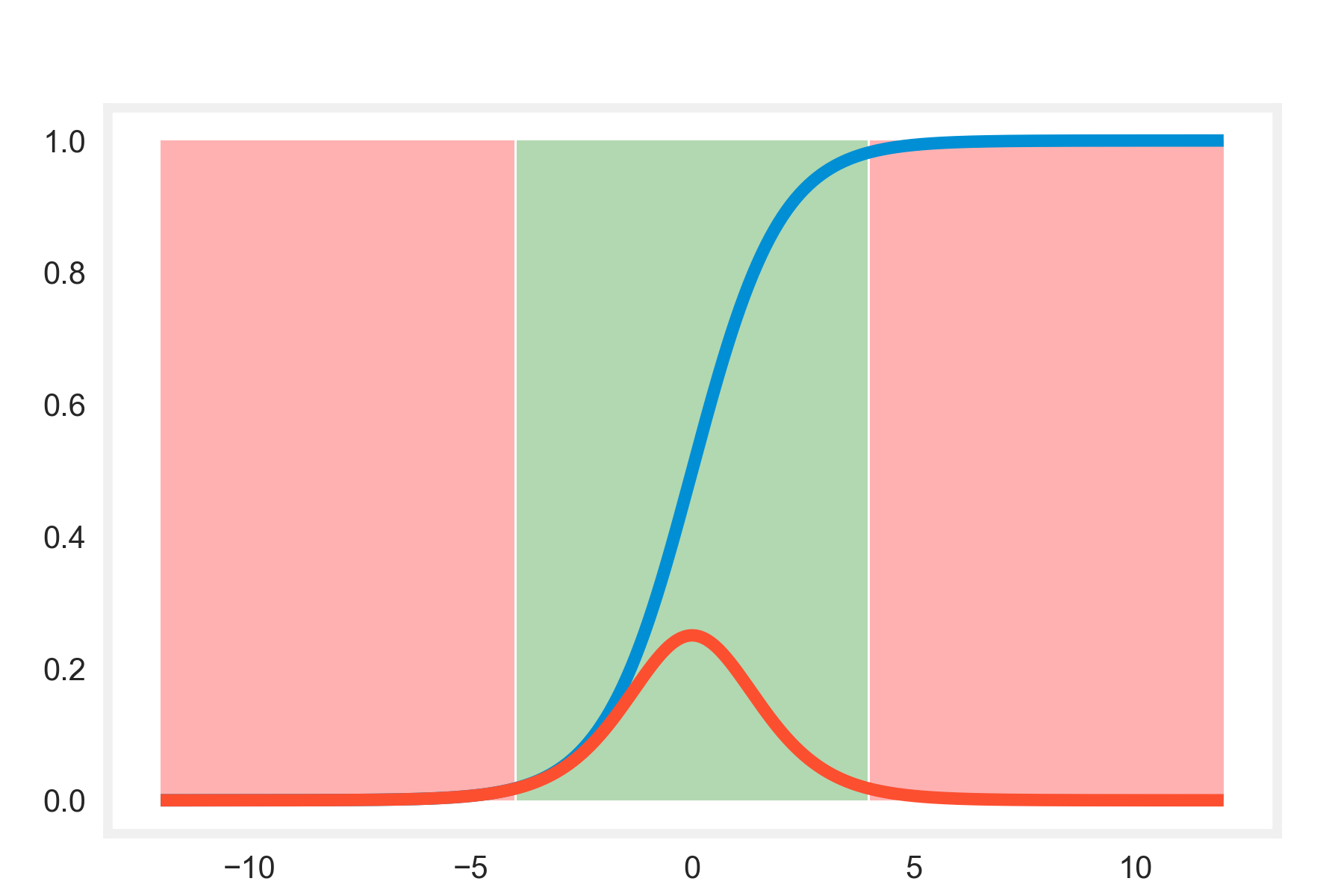
In this plot of the sigmoid activation function (the blue line), and its derivative (red line), you can clearly see the regions of saturation (light red background), where forcing the function to go to zero also forces its derivative to go to zero, causing the vanishing gradients issue as you move back through the layers.

Glorot and Bengio

Xavier Glorot and Yoshua Bengio examined the theoretical effects of weight initialization on the vanishing gradients problem in their 2010 paper¹. The first part of their paper compares activation functions, explaining how certain peculiarities of the commonly-used sigmoid function make it highly susceptible to the problem of saturation, and showing that the hyperbolic tangent and softsign $\left( \frac{x}{1 + |x|} \right)$ activations perform better in this respect.

The second part of their paper considers the problem of initializing weights in a fully connected network, providing theoretical justification for sampling the initial weights from the uniform distribution of a certain variance. The motivating intuition for this is in two parts; for the forward pass, ensuring that the variance of the activations is approximately the same across all the layers of the network allows for information from each training instance to pass through the network smoothly. Similarly, considering the backward pass, relatively similar variances of the gradients allows information to flow smoothly backwards. This ensures that the error data reaches all the layers, so that they can compensate effectively, which is the whole point of training.

Notation and Assumptions

In order to formalize these notions, first we must get some notation out of the way. We have the following definitions:

• $a^L$ is the activation vector for layer $L$, with dimensions $n_L \times 1$, where $n_L$ is the number of units in layer $L$.
• $W^L$ is the matrix of weights for layer $L$, with dimensions $n_L \times n_{L-1}$. Each element $W^L_{jk}$ represents the weight of the connection from neuron $k$ of the current layer to neuron $j$ of the previous one.
• $b^L$ is the bias vector for layer $L$, with the same dimensions as $a^L$.
• $z^L$ is the weighted input to the activation function of layer $L$. This means that $z^L = W^L \times a^{L-1} + b^L$.
• $C$ is the cost function we’re trying to optimize. Glorot and Bengio use the conditional log likelihood $-\log P(y \vert x)$, although the details of this won’t matter much.
• $\sigma$ is the activation function, so that $a^L = \sigma (z^L)$, where the function is applied to each element of the vector.
• $n_L$ is the number of units in layer $L$.
• $x$ is the input vector to the network.
• $\delta^L = \frac{\delta C}{\delta z^L}$ is the gradient of the cost function w.r.t. the weighted inputs of layer $L$, also called the error.

The following analysis holds for a fully connected neural network with $d$ layers, with a symmetric activation function with unit derivative at zero. The biases are initialized to zero, and the activation function is approximated by the identity $f(x) = x$ for the initialization period.

We assume that the weights, activations, weighted inputs, raw inputs to the network, and the gradients all come from independent distributions whose parameters depend only on the layer under consideration. Under this assumption, the common scalar variance of the weights of layer $L$ is represented by $\text{Var}\left[W^L\right]$, with similar representations for the other variables (activations, gradients, etc.)

Forward pass

For the forward pass, we want the layers to keep the input and output variances of the activations equal, so that the activations don’t get amplified or vanish upon successive passes through the layers. Consider $z^L_j$, the weighted input of unit $j$ in layer $L$:

$$\begin{align*} \text{Var}\left[z^L\right] &= \text{Var}\left[z^L_j\right] \\ &= \text{Var}\left[ \sum_{k=0}^{n_{L-1}} W^L_{jk} a^{L-1}_k + b^L_j \right] \\ &= \text{Var}\left[ \sum_{k=0}^{n_{L-1}} W^L_{jk} a^{L-1}_k \right] \\ &= \sum_{k=0}^{n_{L-1}} \text{Var}\left[ W^L_{jk} a^{L-1}_k \right] \\ &= \sum_{k=0}^{n_{L-1}} \text{Var}\left[ W^L_{jk}\right] \text{Var}\left[a^{L-1}_k \right] \\ &= \sum_{k=0}^{n_{L-1}} \text{Var}\left[ W^L \right] \text{Var}\left[a^{L-1} \right] \\ &= n_{L-1} \text{Var}\left[ W^L \right] \text{Var}\left[a^{L-1} \right] \\ \end{align*}$$

In the above simplification, we use the fact that the variance of the sum of two independently random variables is the sum of their variances, under the assumption that the weighted activations would be independent of each other. Later, the variance of the product was expanded out to the product of the variances under the assumption that the weights of the current layer would be independent of the activations of the previous layer. The full expression of the variance of the product of two independent random variables also includes terms containing their means. However, we assume that both activations and weights come from distributions with zero mean, reducing the expression to the product of the variances.

Since the activation function is symmetric, it has value 0 for an input of 0. Furthermore, given that the derivative at 0 is 1, we can approximate the activation function $\sigma$ as the identity during initialization, where the biases are zero and the expected value of the weighted input is zero as well. Under this assumption, $a^{L-1} \approx z^{L-1}$, which reduces the previous expression to the form of a recurrence:

$$\begin{align*} \text{Var}\left[z^L\right] &= n_{L-1} \text{Var}\left[ W^L \right] \text{Var}\left[a^{L-1} \right] \\ &= n_{L-1} \text{Var}\left[ W^L \right] \text{Var}\left[z^{L-1} \right] \\ &= n_{L-1} \text{Var}\left[ W^L \right] n_{L-2} \text{Var}\left[ W^{L-1} \right] \text{Var}\left[z^{L-2} \right] \\ &= \text{Var}\left[ x \right] \prod_{m=0}^{L-1} n_m \text{Var}\left[ W^{m+1} \right] \end{align*}$$

Thus, if we want the variances of all the weighted inputs to be the same, the product term must evaluate to $1$, the easiest way to ensure which is to set $\text{Var}\left[ W^{m+1} \right] = \frac{1}{n_m}$. Written alternatively, for every layer $L$, where $n_\text{in}$ is the number of units to the layer (layer fan-in), we want

$$\text{Var}\left[ W^{L} \right] = \frac{1}{n_\text{in}}$$

Backwards pass

For the backward pass, we want the variances of the gradients to be the same across the layers, so that the gradients don’t vanish or explode prematurely. We use the backpropagation equation as our starting point:

$$\begin{align*} \text{Var}\left[\delta^L\right] &= \text{Var}\left[\delta^L_j\right] \\ &= \text{Var}\left[ \left(\sum_{k=0}^{n_{L+1}} W^{L+1}_{kj} \delta^{L+1}_k \right) \sigma'(z^L_j) \right] \\ &= \text{Var}\left[ \sum_{k=0}^{n_{L+1}} W^{L+1}_{kj} \delta^{L+1}_k \right] \\ &= \sum_{k=0}^{n_{L+1}} \text{Var}\left[ W^{L+1}_{kj} \delta^{L+1}_k \right] \\ &= \sum_{k=0}^{n_{L+1}} \text{Var}\left[ W^{L+1}_{kj} \right] \text{Var}\left[ \delta^{L+1}_k \right] \\ &= \sum_{k=0}^{n_{L+1}} \text{Var}\left[ W^{L+1} \right] \text{Var}\left[ \delta^{L+1} \right] \\ &= n_{L+1} \text{Var}\left[ W^{L+1} \right] \text{Var}\left[ \delta^{L+1} \right] \\ &= n_{L+1} \text{Var}\left[ W^{L+1} \right] n_{L+2} \text{Var}\left[ W^{L+2} \right] \text{Var}\left[ \delta^{L+2} \right] \\ &= \text{Var}\left[ \delta^d \right]\prod_{m=L+1}^{d-1} n_{m} \text{Var}\left[ W^{m} \right] \\ \end{align*}$$

Similarly as in the forwards pass, we assume that the gradients are independent of the weights at initilization, and use the variance identities as explained before. Additionally, we make use of the fact that the weighted input $z^L$ has zero mean during the initialization phase in approximating the derivative of the activation function $\sigma'(z^L_j)$ as $1$. In order to ensure uniform variances in the backwards pass, we obtain the constraint that $\text{Var}\left[W^m\right] = \frac{1}{n_m}$, which can be written in the following form for every layer $L$ and layer fan-out $n_\text{out}$:

$$\text{Var}\left[ W^{L} \right] = \frac{1}{n_\text{out}}$$

Conclusion

In the general case, the fan-in and fan-out of a layer may not be equal, and so as a sort of compromise, Glorot and Bengio suggest using the average of the fan-in and fan-out, proposing that

$$\text{Var}\left[ W^{L} \right] = \frac{2}{n_\text{out} + n_\text{in}}$$

If sampling from a uniform distribution, this translates to sampling the interval $[-a,a]$, where $a = \sqrt{\frac{6}{n_\text{out} + n_\text{in}}}$. The weird-looking $\sqrt{6}$ factor comes from the fact that the variance of a uniform distribution over the interval $[-a,a]$ is $a^2/3$. Alternatively, the weights can be sampled from a normal distribution with zero mean and variance same as the above expression.

Before this paper, the accepted standard initialization technique was to sample the weights from the uniform distribution over the interval $\left[-\frac{1}{\sqrt{n}}, \frac{1}{\sqrt{n}} \right]$, which led to the following variance over the weights: $\text{Var}\left[ W^L \right] = \frac{1}{3n^L}$. Plugging this into the equations we used for the backward pass, it is clear that the gradients decrease as we go backwards through the layers, reducing by about $1/3^\text{rd}$ at each layer, an effect that is borne out experimentally as well. The paper found that the new initialization method suggested ensured that the gradients remained relatively constant across the layers, and this method is now standard for most Deep Learning applications.

It is interesting that the paper makes the assumption of a symmetric activation function with unit derivative at zero, neither of which conditions is satisfied by the logistic activation function. Indeed, the experimental results in the paper (showing unchanging gradients across layers with the new initialization method) are shown with the $tanh$ activation function, which satisfies both assumptions.

For activation functions like ReLU, He et al. work out the required adjustments in their paper². At a high level, since the ReLU function basically zeroes out an entire half of the domain, it should suffice to compensate by doubling the variance of the weights, a heuristic that matches the result of He’s more nuanced analysis, which suggests that $\text{Var}\left[ W^{L} \right] = \frac{4}{n_\text{out} + n_\text{in}}$ works well.

Logistic Activation

In the forward pass derivation, we approximate the activation function as approximately equal to the identity in the initialization phase we are interested in. For the logistic activation function, the equivalent approximation works out to be $\frac{x}{4} + \frac{1}{2}$ (since the derivative at zero is $\frac{1}{4}$ and the value of the function at zero is $\frac{1}{2}$), using a truncated Taylor series expansion around 0. Plugging this in,

$$\begin{align*} \text{Var}\left[z^L\right] &= n_{L-1} \text{Var}\left[ W^L \right] \text{Var}\left[a^{L-1} \right] \\ &= n_{L-1} \text{Var}\left[ W^L \right] \text{Var}\left[\frac{z^{L-1}}{4} + \frac{1}{2} \right] \\ &= n_{L-1} \text{Var}\left[ W^L \right] \text{Var}\left[\frac{z^{L-1}}{4} \right] \\ &= \frac{n_{L-1}}{16} \text{Var}\left[ W^L \right] \text{Var}\left[z^{L-1} \right] \\ \end{align*}$$

The remaining steps are identical, except for the factor $1/16$ in front.

Similarly in the backward pass, where we ignored the derivative of the activation function under the assumption that it was zero, plugging in the correct value of $1/4$ results in a factor of $1/16$ in this case as well.

Together, since this factor of $1/16$ appears identically in both passes, it follows through into the fan-in and fan-out numbers, producing the constraint that

$$\text{Var}\left[ W^{L} \right] = \frac{32}{n_\text{out} + n_\text{in}}$$

Summary of Initialization Parameters

Activation Function	Uniform Distribution $[-a,a]$	Normal distribution
Logistic	$a = 4\sqrt{\frac{6}{n_\text{out} + n_\text{in}}}$	$\sigma = 4\sqrt{\frac{2}{n_\text{out} + n_\text{in}}}$
Hyperbolic Tangent	$a = \sqrt{\frac{6}{n_\text{out} + n_\text{in}}}$	$\sigma = \sqrt{\frac{2}{n_\text{out} + n_\text{in}}}$
ReLU	$a = \sqrt{\frac{12}{n_\text{out} + n_\text{in}}}$	$\sigma = \sqrt{\frac{12}{n_\text{out} + n_\text{in}}}$

References